Month: May 2025

How to Save 1 Million EUR on Electricity in Commercial Buildings – Without the Hassle

Post author By Jana Zazvorkova
Post date May 25, 2025
No Comments on How to Save 1 Million EUR on Electricity in Commercial Buildings – Without the Hassle

Energy savings are a cornerstone of any robust ESG strategy, driving both environmental responsibility and financial performance. At Energy Twin, we leverage advanced AI to seamlessly integrate energy optimization into your building’s operations—delivering substantial cost reductions with minimalized extra workload to your team.

Consider a banking institution with an annual consumption of 50 GWh, where our AI analysis uncovered up to 1 million EUR in potential savings. While each building is unique—some with valid reasons for higher consumption—most branches hide inefficiencies that can be addressed. An AI-driven approach not only reveals these opportunities but also directs your teamon where to focus their efforts. Ultimately, it’s up to you how much of these savings you will be able to implement.

Let’s break down the process into three essential steps:

1. Being Data-Driven

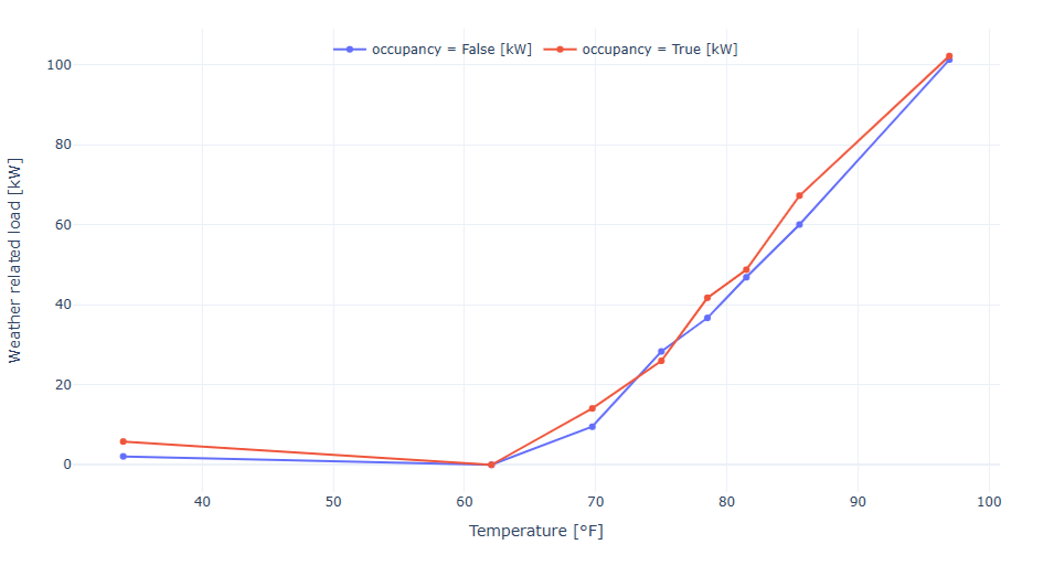
Data is at the heart of effective energy management. Ideally, you’ll have easy, automated access to consumption data—often through APIs and smart meters. Even just the main meter data can reveal surprising inefficiencies thanks to advanced AI algorithms. Of course, the more data you have, the deeper the analysis can go. Additional data points (e.g., sub-meters, HVAC controls, lighting systems) allow for more granular insights and targeted solutions.

2. Continuously Identifying Inefficiencies with AI

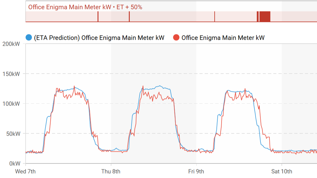
Traditional energy optimization often relies on one-time audits or manual adjustments that quickly become outdated. A modern approach uses continuous data monitoring and advanced AI to:

Uncover Hidden Anomalies: Detect unusual consumption patterns that might be overlooked in manual checks.
Drive Ongoing Optimization: Provide continual recommendations rather than one-off improvements.
Offer Transparent Insights: Deliver unbiased data to help you make clear, objective decisions.

At Energy Twin, we handle the data analysis and AI processes on your behalf. This means minimal additional effort for your team.

3. Incorporating AI Insights into Routine Maintenance

While AI can identify and quantify inefficiencies, the actual savings happen when your technicians or facility managers act on those insights. We recommend:

Regular Meetings: Hold monthly (or bi-weekly) sessions to review AI findings and track progress.
Clear Objectives: Set tangible goals for energy savings and establish timelines for corrective actions.
Team Engagement: Ensure technicians understand both the data and the potential impact of their interventions.

Energy Twin supports you every step of the way with feedback and guidance, but your team is key to turning insights into measurable results.

Ready to Unlock Significant Savings?

By combining AI-driven analysis with proactive facility management, commercial buildings can unlock substantial savings. With Energy Twin’s solution, you gain the insights you need without overburdening your staff or disrupting daily operations.

Interested in learning more about how our platform can help you save on electricity costs? Get in touch with us today for a personalized consultation and find out how easy it can be to start optimizing your building’s energy consumption.

Uncategorized

Decoding Weather-Dependent Loads: Key Patterns and Practical Insights

Post author By Jana Zazvorkova
Post date May 17, 2025
No Comments on Decoding Weather-Dependent Loads: Key Patterns and Practical Insights

In one of our previous posts, we have covered what weather-dependent load is and how it can provide valuable insights into building energy consumption. This week, we’re focusing on specific examples that showcase common weather dependent energy patterns we observe when analyzing buildings.

For all the examples, the x-axis represents outdoor air temperature in °C, and the y-axis shows the additional weather-related energy consumption in kW. The blue line indicates unoccupied regime consumption, while the red line represents occupied regime consumption.

Cooling dominated building

In Figure 1, we see a typical cooling-dominated building with well-managed operations. Notice how energy consumption rises with increasing temperatures only during the occupied regime. During unoccupied periods, the energy consumption remains flat, indicating that the cooling setback is functioning effectively. This is the desired behavior.

However, in Figure 2, we see a different scenario. While there is some distinction between the occupied and unoccupied regimes, the gap is not sufficient to indicate effective cooling setback. This suggests that cooling continues even when the building is unoccupied, revealing energy savings potential.

Heating dominated buildings

The same logic applies to heating-dominated buildings. Heating setbacks during unoccupied periods should be optimized to balance energy savings with thermal inertia. Overly aggressive reductions—such as complete weekend shutdowns—can delay Monday warm-up and strain HVAC systems during recovery. A practical target is an 80% heating setback. For example, if the heating-related load is 10kW, the unoccupied load should ideally be 8kW. Reducing the indoor temperature by just 1°C can lower the heating load by approximately 6%.

Figure 3 demonstrates a heating-dominated building with a well-implemented setback. In contrast, Figure 4 shows a building where heating setback is either nonexistent or poorly implemented, as indicated by the overlapping consumption patterns.

Buildings with Both Heating and Cooling Loads

Of course, a building doesn’t have to be just cooling or heating dominated. Many energy patterns resemble a “U” shape, where we have some heating-related energy consumption in colder months, minimal load during shoulder periods, and cooling-related consumption in warmer months. How should we interpret such patterns, and what should we focus on? Let’s look at a few examples.

In Figure 5, we see a building with both heating and cooling loads, but with almost no distinction between the occupied and unoccupied regimes. The slight reduction in cooling load during unoccupied hours is not sufficient to indicate effective setback implementation. Uncovering immediate savings opportunities can be as easy as reviewing existing equipment schedules and setpoints with no need for costly investment.

In Figure 6, we observe a more defined cooling setback. At 30°C, the unoccupied cooling load is approximately 4kW, while the occupied load is 10kW. However, the heating regime shows minimal differentiation, indicating a missed opportunity to adjust heating schedules and setpoints.

Finally, let’s look at a building that gets it right for both heating and cooling. In Figure 7, we see a clear reduction in the unoccupied regime for both heating and cooling loads. This is the desired behavior, demonstrating effective setbacks and indicating significant potential for savings through targeted schedule and setpoint adjustments.

How can we apply these insights in practice?

Identifying inefficiencies in weather-dependent load patterns provides a clear path to actionable savings. By fine-tuning setpoints and schedules, we can reduce unnecessary consumption, estimate potential savings, and prioritize buildings within a portfolio for targeted adjustments.

Next week, we’ll shift our focus to time-related load patterns and how they shape building energy use. Stay tuned!

Tags Knowledge Base

Uncategorized

Time-of-Week and Temperature model explained

Post author By Jana Zazvorkova
Post date May 12, 2025
No Comments on Time-of-Week and Temperature model explained

Introduction – motivation

Imagine you’re trying to figure out how outside air temperature (OAT) and time-of-week affect energy consumption in a building. With a “common sense” approach, you’d need to test each factor separately—keeping all other variables constant while changing just one. But in the real world, things don’t work that neatly. Inputs like OAT and time-of-week change simultaneously, creating a noisy, messy dataset.

To illustrate this, we’ll use a real-world dataset showing main electricity consumption (kW) alongside OAT (°C). Even at a quick glance, it’s clear that energy use increases during the summer—most likely due to cooling loads. But let’s dig deeper.

In the traditional workflow, analysts often begin by plotting a scatter chart of OAT against energy consumption, using monthly or weekly averages using methods such as degree days or ASHRAE changepoint. However, evaluation of aggregated data does not provide any insight into intraday energy consumption profile. So you need to analyse hourly data. But when we move to hourly data, variability skyrockets, see chart below. For instance, at an OAT of 26 °C during a typical workday, observed consumption can swing anywhere from 60 kW to 130 kW. With such a wide range, pinpointing expected usage becomes nearly impossible without accounting for more than just temperature.

Energy use isn’t driven solely by temperature – it also follows a time-of-week schedule (office hours, weekends, nights). Hot afternoons often coincide with peak operating hours, making it difficult to untangle these overlapping influences. Simply comparing “temperature vs. load” merges two distinct patterns together.

This is where machine-learning models like TOWT come in. By simultaneously fitting both time-of-week and temperature effects, the model learns, for example, that a 30 °C Tuesday at 3 PM will draw more energy not only because it’s hot (cooling demand) but also because it’s mid-afternoon on a workday (higher occupancy).

A helpful analogy is listening to an orchestra. To the untrained ear, it’s a single wall of sound. But experienced listeners can pick out individual instruments, rhythms, and harmonies. TOWT does the same with energy data: it separates overlapping signals so we can understand them in isolation.

Technical detail part

The original concept was introduced by Price in “Methods for Analyzing Electric Load Shape and its Variability” (Lawrence Berkeley National Laboratory Report LBNL-3713E, May 2010) https://eta-publications.lbl.gov/sites/default/files/LBNL-3713E.pdf Since then, it has been widely adopted—cited in numerous academic papers and implemented in open-source tools like RMV2.0 (LBNL), NMECR (kW Engineering), and OpenDSM (formerly OpenEEmeter). It’s also a core part of the CalTRACK Methods and features in several commercial tools, including our own at Energy Twin.

At Energy Twin, we’ve built on the original idea, developing several extensions to make the model more useful in real-world applications—especially where high granularity and robustness are essential.

Weather dependency

Let’s focus on one of those key influences: weather dependency.

Once the TOWT model has separated schedule and temperature effects, we can extract the pure weather-dependent load. This final step reveals how much additional energy consumption is driven specifically by outdoor temperature, plotted separately for occupied and unoccupied days.

By breaking down these intertwined effects, we gain a much clearer understanding of how weather truly impacts energy consumption – a crucial insight when moving from simpler, monthly models to more granular hourly or daily analyses, just compare the graph above with the hourly scatter plot data.

Time-of-Week Dependency

When working with TOWT (Time-Of-Week and Temperature) models, it’s just as important to account for time dependent load – patterns driven not by weather, but by routine. These time-of-week (TOW) driven variations reflect predictable behaviors: office occupancy, operational schedules, or equipment cycles. They repeat week after week, regardless of outdoor conditions.

When modeling the time dependent load – each hour of the week (or 15-minute, 5-minute interval) is treated as a distinct category, allowing the model to capture patterns in energy consumption independently of weather influences. These are typically related to occupancy, schedules, or equipment cycles.

For those who want to dig a bit deeper into the technical side…

To represent these categorical time periods numerically, one-hot encoding (OHC) is used. Using this technique, we transform each time interval into a binary vector where only the element corresponding to the current time slot is set to 1 and all the others are 0. These vectors serve as independent variables in the resulting regression model, enabling it to learn separate baseline consumption levels for each time period. This article provides a clear illustration of how one-hot encoding works, along with simple examples. https://www.geeksforgeeks.org/ml-one-hot-encoding/

Granularity – How precise should your time model be?

The TOWT model reflects multiple levels of temporal granularity, depending on the available data and the desired resolution of analysis. Time-of-week OHC can be constructed at different intervals—such as hourly, 15-minute, or even 5-minute.

Choosing the appropriate resolution is a tradeoff between capturing time-sensitive variability and maintaining model stability. As you can see in graph above, moving from hourly to 15-minute granularity makes a significant difference, revealing much finer operational patterns – such as short-duration spikes or control system behavior.

Variants of TOW Modeling

Each building may require a different definition of the TOW structure, depending on how complex its operational schedule is and how much historical data is available. For facilities with consistent, predictable usage, a simple approach – such as a single daily profile repeated across the week – might be sufficient. But this isn’t suitable for most commercial buildings, which tend to follow more varied routines. A more common approach is the typical TOWT, which assigns a separate profile to each day of the week, allowing the model to reflect different usage on weekdays versus weekends. For even higher fidelity, the model can incorporate custom day types – such as holidays, maintenance periods, or seasonal shutdowns – by adding binary indicators or grouping time slots differently.

Conclusion

The Time-of-Week and Temperature (TOWT) model has become a widely recognized and trusted approach for detailed energy consumption modeling. One of its greatest strengths lies not just in its predictive accuracy, but in its transparency.

Unlike many black-box machine learning models—such as neural networks—that may yield high performance but little interpretability, TOWT offers clear, explainable parameters. These include distinct components for weather-dependent loads and time-of-week-dependent loads, which provide valuable insights into the underlying behavior of a building. In essence, you’re not just getting a forecast—you’re gaining a deeper understanding of how and why a building consumes energy the way it does.

This interpretability is critical in real-world energy analytics, where decision-makers need to justify savings, uncover inefficiencies, and tailor operational strategies based on specific drivers. For example, knowing how much of a building’s load is due to weather (e.g., cooling demand) versus operational schedules (e.g., peak working hours) enables targeted energy-saving measures.

Thanks to its balance between statistical rigor and practical insight, TOWT remains a cornerstone method for analysts, auditors, and engineers working on high-resolution, actionable energy models.

Tags Knowledge Base

Uncategorized

Efficient Multisite Energy Analysis Through AI and Tailored KPIs

Post author By Jana Zazvorkova
Post date May 7, 2025
No Comments on Efficient Multisite Energy Analysis Through AI and Tailored KPIs

AI for Main Electricity Meter Analysis: The Basics

Artificial Intelligence (AI) is revolutionizing energy analysis by turning granular smart meter data into actionable insights. It enables us to detect inefficiencies, forecast usage, and optimize building performance at scale.

This article focuses on analyzing main electricity meters in building portfolios—though the same principles apply to heat, submeters, and other systems. We also highlight the value of explainable AI models that provide both transparency and building-specific insights. Unlike black-box approaches, these tools help users understand and trust the logic behind optimizations.

At the heart of AI-based energy analysis is model identification using historical data. By analyzing a base period, the model learns the typical energy behavior of a building, which can then be used for a variety of applications:

Anomaly Detection: Automatically flagging deviations from expected patterns, whether caused by equipment failures or incorrect schedules.
Energy Conservation Measures (ECMs) Evaluation: Assessing the impact of implemented measures, such as lighting upgrades or HVAC adjustments.
Predictions: Providing accurate energy forecasts for budgeting and operational planning.
Demand Response Scenarios: Simulating and optimizing load reductions during peak demand periods.
Benchmarking: Comparing performance across buildings or time periods to identify underperforming sites.

Various machine learning models can support these tasks, including neural networks, gradient boosting methods like XGBoost, support vector regression, and Time-of-Week and Temperature (TOWT) models. One example builds on TOWT and combines advanced optimization with explainability to deliver deeper, more actionable insights into consumption patterns. This sets the stage for powerful multisite portfolio analysis, with AI scaling insights across hundreds of buildings.

Analyzing Building Portfolios Using Only Main Meter Data

Once AI proves its value at a single site, it’s natural to scale up—because the true power of AI shines when applied across entire building portfolios. By separating weather-dependent and time-dependent loads, AI helps us better understand what drives energy use. And with hundreds of sites, tailored Key Performance Indicators (KPIs) become essential for making sense of the data.

Cooling Setback Insights

In well-managed office buildings, cooling loads should drop significantly when spaces are unoccupied—especially over weekends. Yet, patterns uncovered through AI often reveal something else. Even buildings that appear efficient on paper may show signs of systems running outside expected schedules.

What’s striking is that these insights come from something as simple as main electricity meter data—no extra sensors or submeters needed. It’s a reminder of how much valuable information is already available, waiting to be uncovered through the right lens.

Some common issues include:

Not Integrated Cooling
Cooling systems run independently of actual occupancy, responding only to outdoor temperature. The result: cooling continues over the weekend, even when no one is there.
Overcorrections
Setbacks may be in place but have been manually disabled—often due to Monday morning comfort complaints. For example, cooling a branch on Saturday has little impact on comfort by Monday, but disabling the entire weekend setback wastes energy.
Partial Occupancy, Full Cooling
Only part of the building is in use, but the entire system is cooling as if it were fully occupied.

AI changes the game. With only main meter data, we can uncover hidden inefficiencies, quantify them, and prioritize what matters most.

Consider this: How would you typically find out that a bank branch is cooling over the weekend? No one’s there to notice. There are no complaints. Traditional methods—manual schedule reviews or deploying sensors—are time-consuming, costly, and don’t scale. AI, on the other hand, does scale. It can analyze hundreds of sites automatically and highlight problems in seconds—delivering actionable insights straight to technicians.

Quantifying Performance with KPIs

Spotting inefficiencies is only the beginning. Recognizing problems remotely is helpful—but KPIs make it possible to take action. By translating model outputs into structured, quantifiable metrics, we can benchmark across an entire portfolio and pinpoint the outliers—the “black sheep.”

KPIs help focus attention. Instead of reviewing every building, they steer teams to the ones with the greatest potential for improvement. When a problematic site is flagged, on-site visits can be targeted and efficient—guided by patterns already found in the data.

Real-World KPI Case Study

This approach was applied to a portfolio of 15 buildings, each monitored using 15-minute main meter data.

Step 1: Identifying the Black Sheep

Using historical data, models were trained and evaluated for each site. When KPI comparisons were made, one site clearly stood out. It showed consistently high energy use during nights and weekends—times when the building was expected to be unoccupied. High setback ratios and unusually high base loads raised suspicions of unnecessary cooling during off-hours.

Step 2: On-Site Inspection with Clear Direction

Guided by the data, technicians knew exactly what to look for. At the flagged site, they found that chillers were operating independently of the building management system, running even when no one was there. The site was quickly prioritized for recommissioning.

The result? After reintegrating the chillers into the control system, the building saved 195 MWh annually. The cost savings paid back the investment in less than 12 months.

Conclusion

AI-powered analysis of main meter data offers a scalable, cost-effective way to detect hidden inefficiencies across large portfolios. By combining explainable models with tailored KPIs, we move from raw data to real-world impact—quickly identifying black sheep, prioritizing actions, and delivering measurable results. No extra hardware. No guesswork. Just better decisions, made faster.